Tutorial: Plotting plain electronic band structures

In this tutorial, we explain how to use DFT Hub to generate a plain electronic band structure plot. We use SrTiO₃ as the example system.

Upload the electronic band structure files #

The first step is to upload the required files from your DFT simulation. The upload panel indicates which files can be provided. Not all files are mandatory; however, the file that contains the band information is essential (for example, PROCAR is required for a VASP simulation). In this section, you are also asked to provide the Fermi energy. If the Fermi energy is given, the plot will automatically shift the energies so that the Fermi level is set to zero.

Screenshot of the upload panel indicating the required band-structure files

After selecting the files you can proceed by clicking on the Parse button.

Review generated EBS report cards #

After parsing, the page generates report cards that summarize key results. You can expect values such as bandgap, material type, Fermi value, lattice parameters, angles, volume, and density. If the simulation is spin-polarized and the bandgaps differ between channels, the reports include values for each spin channel.

If you want this report in different units, use the Units panel in the right sidebar.

Electronic report card generated for spin-polarized EBS

Lattice report card generated for spin-polarized EBS

Step 2: Generate a baseline band-structure plot #

Click Plot to render an initial plain-band figure. Use this first result as your baseline before refining limits and styling.

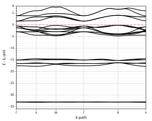
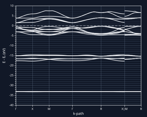
Placeholder image for zoomed plain-band plot

Step 3: Configure the Bandgap tile #

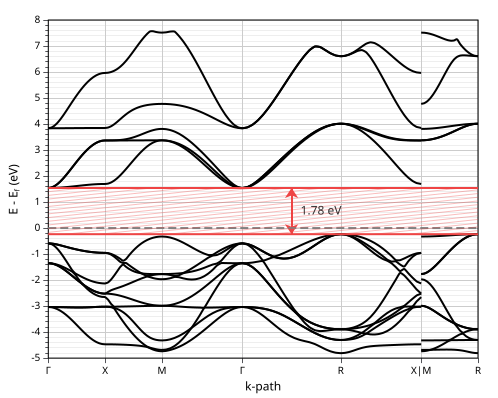
You can use the Bandgap tile to display the band-gap annotation directly on the electronic band-structure plot.

You can enable the annotation by selecting Show bandgap. You can use Line style and Line length to control the separator lines, with length options None, Partial, or Full. You can use Fill style to set the region between the lines to None, Hash, or Solid. In this tutorial, we use Solid line style, Full line length, and Hash fill.

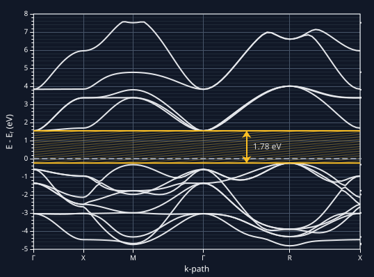
You can also enable Show arrow and Show value to show both the transition direction and the numeric gap value in the rendered figure.

Bandgap tile settings for the plain EBS tutorial

Step 4: Limits #

Limits

To focus on a specific energy range, open Limits in the right sidebar. In this example, set the y-axis range from -6 eV to 8 eV.

You can also set x-limits by high-symmetry-point index: instead of exact k values, provide integers for the starting and ending high-symmetry points.

Click Plot again to update the figure with the zoomed-in window.

Placeholder image for limits sidebar settings in plain EBS tutorial

Use the zoom sliders to focus on specific energy and k-point ranges. Drag slider handles to zoom in or out, and move the selected window to inspect different parts of the band structure.

Placeholder image for plot zoom controls in plain EBS tutorial

Step 5: Customization and styling #

For axis, legend, font, colors, and other appearance controls, use the right sidebar and see the full settings reference in Plot Settings.

Step 6: Export the figure #

When your figure is ready, click the download button in the chart toolbar to export it. Use this to save a clean image for reports, slides, or publications.